Prophet, a forecasting tool created by Facebook, is an open-source solution designed for time series analysis and prediction. Its primary focus is on managing daily observations that exhibit patterns across different time scales. Prophet proves particularly effective in predicting data featuring robust seasonal patterns and multiple seasonalities.
Prophet is available in both Python and R, which makes it a handy choice for many data teams. In this blog, we’ll focus on a step-by-step, Python-only workflow—covering installation, data prep, model fitting, creating future dates, generating forecasts, and reading prediction intervals—so you can follow along in your own notebook from start to finish.
Before getting started, we need to ensure that the Prophet library is installed on our system.
pip install prophet pandas matplotlib
Following the installation process, the script starts by importing pandas as pd, a Python library commonly used for managing and analyzing data, especially when working with structured tables. After that, NumPy is brought in as np to perform numerical operations and handle arrays, which often works hand-in-hand with pandas for data processing tasks. The next line imports the Prophet class from the prophet package, a forecasting library created by Facebook that simplifies the process of modeling and predicting time series data. Lastly, matplotlib.pyplot is imported as plt, a visualization library in Python that allows the creation of plots and charts, which are useful for displaying time series trends, seasonal patterns, and forecast outputs from the Prophet model.
import pandas as pd
import numpy as np
from prophet import Prophet
import matplotlib.pyplot as plt
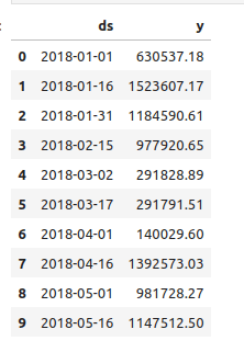
The process begins by importing the sales dataset from a CSV file with pandas. Once the dataset is loaded, the relevant columns are renamed to 'ds' and 'y,' which are the default names required by Prophet for time series forecasting. Here, 'ds' refers to the date field, while 'y' holds the numeric values, such as sales figures, that we aim to predict. Next, the 'ds' column is converted into a datetime format to make sure time-based operations are handled accurately. As a final step, the first few rows of the dataset are displayed with head(10) to confirm that the data has been properly structured and formatted.
df = pd.read_csv('sales_data.csv')
df = df.rename(columns={'date': 'ds', 'sales': 'y'})
df['ds'] = pd.to_datetime(df['ds'])
df.head(10)
Output:
model = Prophet()
model.fit(df)
The model is fitted by creating a new instance of the Prophet object. Configuration settings for the forecasting process are specified in the constructor. Subsequently, the fit method is invoked, and the historical data frame is provided as an input. The fitting process is expected to be completed within 1–5 seconds.
future = model.make_future_dataframe(periods=365)
future.tail(10)
Before generating forecasts, we need to extend our dataset with future dates. This is handled by Prophet’s make_future_dataframe() function. When we pass periods=365, the model appends an extra 365 days to the existing timeline, giving us one full year of dates to base predictions on. After creating these new entries, we use future.tail(10) to display the last 10 rows. This quick check ensures that the future dates have been added correctly and confirms that the dataset is ready for forecasting.
Output:
forecast = model.predict(future)
forecast[['ds', 'yhat', 'yhat_lower', 'yhat_upper']].tail(10)
In this step, we use the Prophet model’s predict() function on the future dates we prepared, which produces a forecast DataFrame containing the model’s predictions. This DataFrame not only holds the expected values but also includes uncertainty ranges to account for variability in the forecast. To focus on the key information, we extract the columns ds (date), yhat (the predicted value), and yhat_lower and yhat_upper (the lower and upper limits of the confidence interval). By applying .tail(), we view the last few records of this dataset, which helps us verify the projected values and their associated ranges. This step is valuable because it provides both a central forecast and a realistic spread of possible outcomes, highlighting the uncertainty that naturally exists in time series predictions.
Output:
fig1 = model.plot(forecast)
plt.title('Sales Forecast')
plt.xlabel('Date')
plt.ylabel('Sales')
plt.grid(True)
# Plot components
fig2 = model.plot_components(forecast)
plt.show()
In this step, we move on to visualizing the forecast produced by the Prophet model. The function model.plot(forecast) generates a time series chart that combines the historical observations with the model’s predicted values, while additional formatting such as a title, axis labels, and a grid is added for better readability. To further explore the behavior of the data, model.plot_components(forecast) is used, which separates the forecast into different elements like the overall trend, seasonal effects, and weekly patterns, helping us understand what influences the predictions. Finally, the plt.show() command is executed to render these plots, giving a clear visual overview of the forecasting results.
Output:
This is the graphical representation of the generated forecast.
This is the Trend and Seasonality for a Year.
To sum up, Prophet provides an easy-to-use yet highly effective way to perform time series forecasting in Python. By following the process of preparing data, training the model, extending the timeline, generating predictions, and visualizing results, we can build insightful forecasts with ease. Its strength in capturing seasonality, trends, and uncertainty makes it a valuable tool for analysts and businesses seeking reliable and actionable predictions.
To read more about Getting Started with the Requests Library in Python, refer to our blog Getting Started with the Requests Library in Python.