SciPy, an abbreviation for Scientific Python, is an open-source library built on top of NumPy, another fundamental Python library for numerical computing. It extends NumPy's capabilities and provides a vast array of modules and functions that are essential for high-level scientific computing tasks. SciPy includes optimized and added functions that are frequently used in NumPy and Data Science.
To install SciPy, run the following command:
pip install scipy
After installing SciPy, you can import any modules in SciPy. SciPy's collection of modules serves as a valuable resource, providing a wide array of tools tailored for different applications and tasks. Let's explore the array of modules within SciPy.
Constants in SciPy
SciPy offers a range of predefined scientific constants that serve as valuable tools, especially in Data Science tasks.
The scipy.constants module in SciPy organizes different types of essential numbers into easy-to-find groups. These groups include numbers related to how things work in the physical world (like speed of light and gravity), properties of tiny particles (atoms and nuclei), and important mathematical values (such as p and e). If someone needs to know the value of the speed of light or the mathematical constant p for a scientific calculation, they can easily find these values without searching elsewhere.
To access the mathematical constant p (pi) using the constants module:
from scipy import constants
print(constants.pi)    # Output: 3.141592653589793
Mass
In SciPy's constants module, you can access various fundamental constants related to mass. These constants provide values for masses of fundamental particles such as electrons, protons, and neutrons, as well as units like the atomic mass unit and atomic mass constant. They can be utilized in various scientific computations, especially in physics, chemistry, nuclear physics, and related fields where precise mass values are required for calculations or analysis.
Here are some of the mass-related constants available in the constants module of SciPy:
from scipy import constants
print(constants.atomic_mass)            # 1.6605390666e-27
print(constants.m_u)                    # 1.6605390666e-27
print(constants.electron_mass)          # 9.1093837015e-31
print(constants.proton_mass)            # 1.67262192369e-27
print(constants.neutron_mass)           # 1.67492749804e-27
print(constants.m_n)                    # 1.67492749804e-27
print(constants.m_p)                    # 1.67262192369e-27
print(constants.gram)                   # 0.001
print(constants.metric_ton)             # 1000.0
print(constants.grain)                  # 6.479891e-05
print(constants.lb)                     # 0.45359236999999997
print(constants.pound)                 # 0.4535923699999999
print(constants.oz)                    # 0.028349523124999998
print(constants.ounce)                 # 0.028349523124999998
print(constants.stone)                 # 6.3502931799999995
print(constants.long_ton)              # 1016.0469088
print(constants.short_ton)             # 907.1847399999999
print(constants.troy_ounce)            # 0.031103476799999998
print(constants.troy_pound)            # 0.37324172159999996
print(constants.carat)                 # 0.0002
Metric (SI) Prefixes
In SciPy's constants module, you can find the Metric (SI) prefixes that represent various powers of 10 used for denoting decimal multiples and submultiples of units. These prefixes enable easier representation of extremely large or small quantities in scientific computations and measurements.
from scipy import constants
print(constants.yotta)    #1e+24
print(constants.zetta)    #1e+21
print(constants.exa)      #1e+18
print(constants.peta)     #1000000000000000.0
print(constants.tera)     #1000000000000.0
print(constants.giga)     #1000000000.0
print(constants.mega)     #1000000.0
print(constants.kilo)     #1000.0
print(constants.hecto)    #100.0
print(constants.deka)     #10.0
print(constants.deci)     #0.1
print(constants.centi)    #0.01
print(constants.milli)    #0.001
print(constants.micro)    #1e-06
print(constants.nano)     #1e-09
print(constants.pico)     #1e-12
print(constants.femto)    #1e-15
print(constants.atto)     #1e-18
print(constants.zepto)    #1e-21
Binary Prefixes
SciPy's constants module includes Binary Prefixes, representing powers of 2 that are widely used in computing to denote binary multiples or submultiples of bytes. These prefixes offer a convenient way to express data storage capacities in the realm of digital information.
from scipy import constants
print(constants.kibi)    #1024
print(constants.mebi)    #1048576
print(constants.gibi)    #1073741824
print(constants.tebi)    #1099511627776
print(constants.pebi)    #1125899906842624
print(constants.exbi)    #1152921504606846976
print(constants.zebi)    #1180591620717411303424
print(constants.yobi)    #1208925819614629174706176
Angle
SciPy provides various functions and constants for working with angles in radians and degrees. The constants module includes some essential angle-related constants like pi, which represents p (pi), and the radian and degree constants, which represent conversion factors between radians and degrees.
from scipy import constants
print(constants.degree)     #0.017453292519943295
print(constants.arcmin)     #0.0002908882086657216
print(constants.arcminute)  #0.0002908882086657216
print(constants.arcsec)     #4.84813681109536e-06
print(constants.arcsecond)  #4.84813681109536e-06
Time
SciPy provides various constants for working with time.
from scipy import constants
print(constants.minute)      #60.0
print(constants.hour)        #3600.0
print(constants.day)         #86400.0
print(constants.week)        #604800.0
print(constants.year)        #315364000.0
print(constants.Julian_year) #31557600.0
Length
The constants module provides various constants related to length, offering conversion factors and fundamental lengths used in scientific computations. These constants allow users to work with different units of length and perform conversions between them.
from scipy import constants
print(constants.inch)             #0.0254
print(constants.foot)             #0.30479999999999996
print(constants.yard)             #0.9143999999999999
print(constants.mile)             #1609.3439999999998
print(constants.mil)              #2.5399999999999997e-05
print(constants.pt)               #0.00035277777777777776
print(constants.point)            #0.00035277777777777776
print(constants.survey_foot)      #0.3048006096012192
print(constants.survey_mile)      #1609.3472186944373
print(constants.nautical_mile)    #1852.0
print(constants.fermi)            #1e-15
print(constants.angstrom)         #1e-10
print(constants.micron)           #1e-06
print(constants.au)               #149597870691.0
print(constants.astronomical_unit) #149597870691.0
print(constants.light_year)       #9460730472580800.0
print(constants.parsec)           #3.0856775813057292e+16
Pressure
In the constants module, there are several constants related to pressure. These constants provide conversion factors between different units of pressure and offer fundamental pressure values used in scientific computations.
from scipy import constants
print(constants.atm)         #101325.0
print(constants.atmosphere)  #101325.0
print(constants.bar)         #100000.0
print(constants.torr)        #133.32236842105263
print(constants.mmHg)        #133.32236842105263
print(constants.psi)         #6894.757293168361
Area
In the constants module, there are several constants related to area.
from scipy import constants
print(constants.hectare) #10000.0
print(constants.acre)    #4046.8564223999992
Volume
In the constants module, there are several constants related to volume.
from scipy import constants
print(constants.liter)            #0.001
print(constants.litre)            #0.001
print(constants.gallon)           #0.0037854117839999997
print(constants.gallon_US)        #0.0037854117839999997
print(constants.gallon_imp)       #0.00454609
print(constants.fluid_ounce)      #2.9573529562499998e-05
print(constants.fluid_ounce_US)   #2.9573529562499998e-05
print(constants.fluid_ounce_imp)  #2.84130625e-05
print(constants.barrel)           #0.15898729492799998
print(constants.bbl)              #0.15898729492799998
Speed
In SciPy's constants module, you can find constants related to speed, providing conversion factors between different units of speed and essential speed values used in scientific computations.
from scipy import constants
print(constants.kmh)            #0.2777777777777778
print(constants.mph)            #0.44703999999999994
print(constants.mach)           #340.5
print(constants.speed_of_sound) #340.5
print(constants.knot)           #0.5144444444444445
Temperature
SciPy provides various constants related to temperature.
from scipy import constants
print(constants.zero_Celsius)      #273.15
print(constants.degree_Fahrenheit) #0.5555555555555556
Sparse Data in SciPy
Sparse data refers to datasets or matrices that contain a vast number of zero elements relative to the total number of elements. In scientific computing and data analysis, dealing with sparse data is crucial due to its prevalence in various fields, including machine learning, scientific simulations, and network analysis.
Scipy includes a submodule called scipy.sparse that provides functionalities to work efficiently with sparse data structures. These data structures optimize memory usage by storing only the nonzero elements along with their indices, which significantly reduces storage requirements and computational overhead compared to storing dense matrices where most values are zeros.
Scipy offers several types of sparse matrices, such as
* CSC (Compressed Sparse Column): This format stores the sparse matrix by column, where each column is represented as three one-dimensional arrays - one for nonzero values, one for row indices, and another for column pointers.
* CSR (Compressed Sparse Row): Similar to CSC, this format stores the matrix by rows, making it more efficient for row-based operations.
* COO (Coordinate Format): Here, the sparse matrix is represented using three arrays containing the row indices, column indices, and values of nonzero elements.
import numpy as np
from scipy.sparse import csc_matrix
# Creating a dense matrix
dense_matrix = np.array([[0, 0, 3], [4, 0, 0], [0, 5, 6]])
# Converting the dense matrix to a CSC sparse matrix
sparse_matrix_csc = csc_matrix(dense_matrix)
# Accessing elements of the CSC sparse matrix
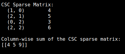
print("CSC Sparse Matrix:")
print(sparse_matrix_csc)
# Performing operations on the CSC sparse matrix
col_sum = sparse_matrix_csc.sum(axis=0)
print("\nColumn-wise sum of the CSC sparse matrix:")
print(col_sum)
Output:
Spatial Data in SciPy
Scipy includes modules that provide functionalities for working with spatial data and performing various spatial operations. Spatial data refers to information associated with geographical or spatial locations, commonly used in geographic information systems (GIS), mapping, and analysis of spatial relationships.
The scipy.spatial module within Scipy offers tools and algorithms for handling and processing spatial data. It provides a range of functionalities useful for computational geometry, distance calculations, spatial transformations, and nearest neighbor computations, among others.
Key components and functionalities of the scipy.spatial module includes:
Distance Calculations: Scipy offers methods to compute distances between points in different dimensions using various metrics such as Euclidean distance, Manhattan distance, Minkowski distance, and more. This is particularly useful in spatial analysis, clustering, and classification tasks.
Spatial Convex Hull: The module provides algorithms to compute the convex hull of a set of points in space. Convex hulls are fundamental in understanding the shape and structure of spatial data points.
An example illustrating the usage of some functionalities from scipy.spatial:
import numpy as np
from scipy.spatial.distance import euclidean, cityblock, minkowski
from scipy.spatial import ConvexHull
# Example of distance calculation between two points
point1 = (1, 2)
point2 = (4, 6)
# Euclidean distance calculation
euclidean_dist = euclidean(point1, point2)
print(euclidean_dist)              # Output: 5.0
# Manhattan distance calculation
cityblock = cityblock(point1, point2)
print(cityblock)                 # Output: 7
# Minkowski distance calculation
minkowski_dist = minkowski(point1, point2, p=3)
print(minkowski_dist)             # Output: 4.497941445275415
# Computing the convex hull of a set of points
points = np.array([[0, 0], [1, 1], [1, 0], [0, 1]])
hull = ConvexHull(points)
print(hull.vertices)             # Output: [0 2 1 3]
SciPy Graphs
Scipy includes functionalities for working with graphs and networks through its scipy.sparse.csgraph module. It provides tools to create, manipulate, and analyze graphs efficiently.
Key functionalities of scipy.sparse.csgraph for working with graphs include:
1. Shortest Path Algorithms: These include various algorithms to compute shortest paths between nodes in a graph. Algorithms like Dijkstra's algorithm, Floyd-Warshall algorithm, and Bellman-Ford algorithm are available for finding shortest paths considering different scenarios.
* Dijkstra's algorithm
It takes the below arguments:
return_predecessors: boolean (True to return entire path of traversal otherwise False).
indices: the element's index, which returns all paths leading to that element alone.
limit: the path's maximum weight.
import numpy as np
from scipy.sparse.csgraph import dijkstra
from scipy.sparse import csr_matrix
arr =  np.array([
    [0, 4, 0],
    [0, 0, 8],
    [0, 0, 7]])
newarr = csr_matrix(arr)
print(dijkstra(newarr, return_predecessors=True, indices=0))
Output: (array([0., 1., 2.]), array([-9999, 0, 0], dtype=int32))
* Floyd-Warshall algorithm
import numpy as np
from scipy.sparse.csgraph import floyd_warshall
from scipy.sparse import csr_matrix
arr = np.array([
  [0, 1, 2],
  [1, 3, 0],
  [2, 1, 3]
])
newarr = csr_matrix(arr)
print(floyd_warshall(newarr, return_predecessors=True))
Output: (array([[0., 1., 2.], [1., 0., 3.], [2., 1., 0.]]),
array([[-9999,     0,     0], [    1, -9999,     0],[    2,     2, -9999]], dtype=int32))
Bellman-Ford algorithm
import numpy as np
from scipy.sparse.csgraph import bellman_ford
from scipy.sparse import csr_matrix
arr = np.array([
  [0, -1, 2],
  [1, 0, 7],
  [2, 1, 3]
])
newarr = csr_matrix(arr)
print(bellman_ford(newarr, return_predecessors=True, indices=0))
Output: (array([ 0., -1., 2.]), array([-9999, 0, 0], dtype=int32))
2. Connected Components: Scipy provides functions to find connected components within a graph. This is essential in understanding the structure and connectivity of networks.
import numpy as np
from scipy.sparse.csgraph import connected_components
from scipy.sparse import csr_matrix
arr = np.array([
  [0, 1, 2],
  [1, 0, 0],
  [2, 0, 0]
])
newarr = csr_matrix(arr)
print(connected_components(newarr))
Output: (1, array([0, 0, 0], dtype=int32))
Interpolation
Interpolation in Scipy refers to the process of estimating values between known data points. For example, we could interpolate between points 1 and 2 to obtain points 1.44 and 1.66.
Scipy provides various interpolation methods to perform this task efficiently.
The scipy.interpolate submodule offers a wide range of functions and classes for interpolation, catering to different types of data and requirements. Some commonly used interpolation methods available in Scipy include:
1. Linear Interpolation (interp1d): This method constructs a linear interpolating function between data points. It assumes a linear relationship between consecutive points.
from scipy.interpolate import interp1d
import numpy as np
xs = np.array([1,2,3,4,5,6,7,8,9])
ys = 2*xs + 1
interp_func = interp1d(xs, ys)
newarr = interp_func(np.arange(2.1, 3, 0.1))
print(newarr)
Output: [5.2 5.4 5.6 5.8 6. 6.2 6.4 6.6 6.8]
Spline Interpolation: Spline interpolation constructs piecewise cubic polynomials between data points, ensuring smoothness by maintaining continuity in the first and second derivatives.
from scipy.interpolate import UnivariateSpline
import numpy as np
xs = np.array([1,2,3,4,5,6,7,8,9])
ys = xs**2 + np.sin(xs) + 1
interp_func = UnivariateSpline(xs, ys)
newarr = interp_func(np.arange(2.1, 3, 0.1))
print(newarr)
Output: [5.62894853 5.9917962 6.37883473 6.78997537 7.22512936 7.68420794 8.16712235 8.67378384 9.20410364]
These are some of the important modules provided by SciPy. Scipy stands as a robust and versatile library in Python's scientific computing ecosystem, offering an extensive array of tools and functions for various numerical and scientific tasks. With its powerful capabilities, Scipy simplifies complex computations and enables researchers, scientists, and developers to tackle a wide range of scientific problems efficiently.